Speed Planning Problem - Basic Model

In this example, we demonstrate how to use OPTIMake to model and solve a multi-stage problem, such as a trajectory planning problem or an MPC control problem.

Problem Description

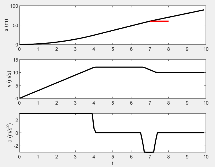
Consider a 10 s speed planning problem where we need the speed to reach a given reference speed $v_{ref}$. Additionally, we need to consider the following constraints:

• Acceleration is limited to [-3, 3] $m/s^2$
• Initial position is 0 $m$, initial speed is 0 $m/s$
• The position must be greater than 60 $m$ within the [7, 8] s time window

Based on the above problem setup, we define the following objective function:

$$\min \sum_{i=1}^{N} (v_i - v_{ref})^2$$

Additionally, we need to consider the following constraints:

$$\begin{split} &\dot{s} = v \\ &\dot{v} = a \\ &s(0) = 0 \\ &v(0) = 0 \\ &s(t) \geq 60, t \in [7, 8] \\ &a \in [-3, 3] \end{split}$$

Modeling

The above optimization problem is modeled in OPTIMake as follows.

We divide the 10 s time window into 100 time points, i.e., $N=100$ (corresponding to a time step of 0.1 s).

prob = multi_stage_problem('speed_planning', 100)

Next, we need to define the problem parameters: the speed reference value $v_{ref}$ and the position lower bound $s_{min}$. Since $s_{min}$ is a time-dependent parameter, we need to define it as a stage-dependent parameter, meaning a different value can be set at each stage (time point).

vref = prob.parameter('vref',  stage_dependent=False)
smin = prob.parameter('smin',  stage_dependent=True)

Then, we need to define the problem variables $s$, $v$, and $a$. Note that when defining variables, we can simultaneously set the upper and lower bounds (hard bounds and soft bounds) for the variable. For example, we can set the lower bound of $s$ to $s_{min}$, and the bounds of $a$ to [-3, 3].

s = prob.variable('s', hard_lowerbound=smin)
v = prob.variable('v')
a = prob.variable('a', hard_lowerbound=-3, hard_upperbound=3)

Next, we need to define the objective function. Here we use the general_objective function to define it.

obj = general_objective((v - vref)**2)
prob.objective(obj)

Next, we need to define the constraints. Here we use the differential_equation function to define the state equation. Note that when defining the state equation, we need to set the time step (i.e., the discretization step size). Here we use the 4th-order Runge-Kutta method to discretize the state equation.

ode = differential_equation(
    state=[s, v],
    state_dot=[v, a], 
    stepsize=0.1, 
    discretization_method='erk4')
prob.equality(ode)

Alternatively, when the state equation is in discrete form, we can use the discrete_equation function to define it. For example, we can discretize the state equation as follows ($h$ is the time step):

$$\begin{split} &s_{i+1} = s_i + h v_i + \frac{1}{2} h^2 a_i \\ &v_{i+1} = v_i + h a_i \\ \end{split}$$

The code using the discrete_equation function to define the state equation constraint is as follows:

h = 0.1
dis_eq = discrete_equation(
    expr_next_stage=[s, v],
    expr_this_stage=[s + h * v + 0.5 * h**2 * a, v + h * a]
)
prob.equality(dis_eq)

Next, we need to define the initial conditions. Here we use the start_equality function.

seq = general_equality([s - 0, v - 0])
prob.start_equality(seq)

After completing the above modeling, we can generate the code:

option = codegen_option()
codegen = code_generator()
codegen.codegen(prob, option)

The complete code is as follows:

prob = multi_stage_problem('speed_planning', 100)
vref = prob.parameter('vref',  stage_dependent=False)
smin = prob.parameter('smin', stage_dependent=True)

s = prob.variable('s', hard_lowerbound=smin)
v = prob.variable('v')
a = prob.variable('a', hard_lowerbound=-3, hard_upperbound=3)

obj = general_objective((v - vref)**2)
prob.objective(obj)

# use differential equation to define the state equation
ode = differential_equation(
    state=[s, v],
    state_dot=[v, a], 
    stepsize=0.1, 
    discretization_method='erk4')
prob.equality(ode)

# alternative way to define the state equation
# h = 0.1
# dis_eq = discrete_equation(
#     expr_next_stage=[s, v],
#     expr_this_stage=[s + h * v + 0.5 * h**2 * a, v + h * a]
# )
# prob.equality(dis_eq)

seq = general_equality([s - 0, v - 0])
prob.start_equality(seq)

option = codegen_option()
codegen = code_generator()
codegen.codegen(prob, option)

Solving

Below is the code for calling the solver using C/C++.

#include "speed_planning_prob.h"
#include "speed_planning_solver.h"
#include <stdio.h>

int main(void)
{
    Speed_planning_Problem prob;
    Speed_planning_Option option;
    Speed_planning_WorkSpace ws;
    Speed_planning_Output output;
    speed_planning_init(&prob, &option, &ws);

    /* params */
    prob.param[SPEED_PLANNING_PARAM_VREF] = 10.0; /* vref */
    for (size_t i = 0; i < SPEED_PLANNING_DIM_N; i++) {
        /* smin */
        if ((i >= 70) && (i <= 80)) {
            prob.param_stage[i][SPEED_PLANNING_PARAM_STAGE_SMIN] = 60.0;
        } else {
            prob.param_stage[i][SPEED_PLANNING_PARAM_STAGE_SMIN] = 0.0;
        }
    }
    
    /* option */
    int solve_status = speed_planning_solve(&prob, &option, &ws, &output);
    
    printf("solve_status = %d\n", solve_status);
    return 0;
}

Results