Minimum Time-to-Climb Problem

Problem Description

This example solves the classical minimum time-to-climb problem for the Bryson aircraft, adapted from the GPOPS-II benchmark. The aircraft starts from sea level with a prescribed initial speed, mass, and zero flight-path angle, and must reach a target altitude and terminal speed in level flight while minimizing the final time.

This example is mainly used to demonstrate the following features of OPTIMake:

• lookup_table interpolation for data-driven modeling
• scaling of optimization variables for improved numerical conditioning

The performance index is

$$J = t_f$$

The state variables are altitude $h$, speed $v$, flight-path angle $\gamma$, and mass $m$. The control variable is the angle of attack $\alpha$. The equations of motion used in the example are

$$\begin{split} \dot{h} &= v \sin \gamma \\ \dot{v} &= \frac{T \cos \alpha - D}{m} - \frac{\mu}{r^2} \sin \gamma \\ \dot{\gamma} &= \frac{T \sin \alpha + L}{m v} + \left(\frac{v}{r} - \frac{\mu}{v r^2}\right) \cos \gamma \\ \dot{m} &= -\frac{T}{g_0 I_{sp}} \end{split}$$

with

$$r = R_e + h$$

The aerodynamic and propulsion terms are computed from lookup tables:

$$\begin{split} M &= \frac{v}{a(h)} \\ C_D &= C_{D0}(M) + \eta(M) C_{L_\alpha}(M) \alpha^2 \\ C_L &= C_{L_\alpha}(M) \alpha \\ q &= \frac{1}{2} \rho(h) v^2 \\ D &= q S C_D \\ L &= q S C_L \\ T &= T(M, h) \end{split}$$

Here, this model contains five 1D lookup tables for $a(h)$, $\rho(h)$, $C_{D0}(M)$, $C_{L_\alpha}(M)$, $\eta(M)$, and one 2D lookup table for $T(M, h)$:

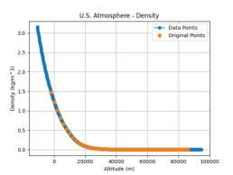
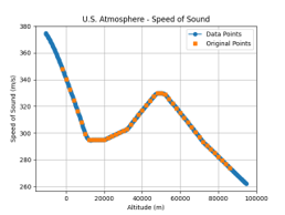
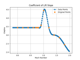
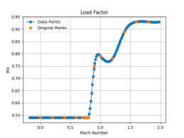
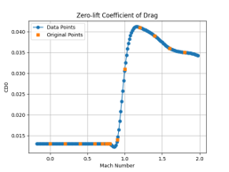
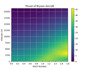
The example also imposes box constraints on final time, altitude, speed, flight-path angle, mass, and angle of attack. In the implementation, these variables are scaled before optimization to improve numerical conditioning.

信息

This example is a good reference when a flight mechanics model depends on 1-D and 2-D lookup tables. OPTIMake combines lookup_table interpolation with the optimal control transcription directly, so atmospheric density, speed of sound, thrust, and aerodynamic coefficients can be used in the model without manually fitting simplified analytic expressions.

Modeling

The full Python script first defines the atmosphere, thrust, and aerodynamic tables, then builds the optimal control problem. The core modeling part is shown below.

NN = 100
prob = multi_stage_problem('mintime2climb', NN + 1)

tfmin, tfmax = 100, 800
altmin, altmax = 0, 21031.2
speedmin, speedmax = 5, 1000
fpamin, fpamax = -40 * pi / 180, 40 * pi / 180
massmin, massmax = 22, 20410
alphamin, alphamax = -pi / 4, pi / 4

tf_scaling = 1000.0
alt_scaling = 10000.0
speed_scaling = 1000.0
fpa_scaling = 1.0
mass_scaling = 10000.0
alpha_scaling = 1.0

h_s = prob.variable('h_s', hard_lowerbound=altmin / alt_scaling, hard_upperbound=altmax / alt_scaling)
v_s = prob.variable('v_s', hard_lowerbound=speedmin / speed_scaling, hard_upperbound=speedmax / speed_scaling)
fpa_s = prob.variable('fpa_s', hard_lowerbound=fpamin / fpa_scaling, hard_upperbound=fpamax / fpa_scaling)
m_s = prob.variable('m_s', hard_lowerbound=massmin / mass_scaling, hard_upperbound=massmax / mass_scaling)
alpha_s = prob.variable('alpha_s', hard_lowerbound=alphamin / alpha_scaling, hard_upperbound=alphamax / alpha_scaling)
tf_s = prob.variable('tf_s', hard_lowerbound=tfmin / tf_scaling, hard_upperbound=tfmax / tf_scaling)

h = alt_scaling * h_s
v = speed_scaling * v_s
fpa = fpa_scaling * fpa_s
m = mass_scaling * m_s
alpha = alpha_scaling * alpha_s
tf = tf_scaling * tf_s

mu = 3.986e14
S = 49.2386
g0 = 9.80665
Isp = 1600
Re = 6378145

# data with denser points for M<=0.8
M2         = [0, 0.2, 0.4, 0.6, 0.7, 0.75, 0.78, 0.8, 0.9, 1.0, 1.2, 1.4, 1.6, 1.8]
Clalphatab = [3.44, 3.44, 3.44, 3.44, 3.44, 3.44, 3.44, 3.44, 3.58, 4.44, 3.44, 3.01, 2.86, 2.44]
CD0tab     = [0.013, 0.013, 0.013, 0.013, 0.013, 0.013, 0.013, 0.013, 0.014, 0.031, 0.041, 0.039, 0.036, 0.035]
etatab     = [0.54, 0.54, 0.54, 0.54, 0.54, 0.54, 0.54, 0.54, 0.75, 0.79, 0.78, 0.89, 0.93, 0.93]

lt_Clalpha = lookup_table(name='Clalpha', points=M2, values=Clalphatab, method='cubic', bc_type='natural')
lt_CD0 = lookup_table(name='CD0', points=M2, values=CD0tab, method='cubic', bc_type='natural')
lt_eta = lookup_table(name='eta', points=M2, values=etatab, method='cubic', bc_type='natural')

Mtab   = np.array(
    [0, 0.2, 0.4, 0.6, 0.8, 1, 1.2, 1.4, 1.6, 1.8])
alttab = 304.8 * np.array(
    [0, 5, 10, 15, 20, 25, 30, 40, 50, 70])
Ttab   = 4448.222* np.array(
    [[24.2, 24.0, 20.3, 17.3, 14.5, 12.2, 10.2,  5.7,  3.4, 0.1], # M = 0
    [28.0, 24.6, 21.1, 18.1, 15.2, 12.8, 10.7,  6.5,  3.9, 0.2], # M = 0.2
    [28.3, 25.2, 21.9, 18.7, 15.9, 13.4, 11.2,  7.3,  4.4, 0.4],
    [30.8, 27.2, 23.8, 20.5, 17.3, 14.7, 12.3,  8.1,  4.9, 0.8],
    [34.5, 30.3, 26.6, 23.2, 19.8, 16.8, 14.1,  9.4,  5.6, 1.1],
    [37.9, 34.3, 30.4, 26.8, 23.3, 19.8, 16.8, 11.2,  6.8, 1.4],
    [36.1, 38.0, 34.9, 31.3, 27.3, 23.6, 20.1, 13.4,  8.3, 1.7],
    [36.1, 36.6, 38.5, 36.1, 31.6, 28.1, 24.2, 16.2, 10.0, 2.2],
    [36.1, 35.2, 42.1, 38.7, 35.7, 32.0, 28.1, 19.3, 11.9, 2.9],
    [36.1, 33.8, 45.7, 41.3, 39.8, 34.6, 31.1, 21.7, 13.3, 3.1]])
lt_T = lookup_table(name='T', points=[Mtab.tolist(), alttab.tolist()], values=Ttab.tolist(), method='cubic') 


r = Re + h
rho = interpolation(lt_us1976_density, h)
sos = interpolation(lt_us1976_sos, h)
Mach = v / sos
Thrust = interpolation(lt_T, Mach, h)


CD0 = interpolation(lt_CD0, Mach)
Clalpha = interpolation(lt_Clalpha, Mach)
eta = interpolation(lt_eta, Mach)

CD = CD0 + eta * Clalpha * alpha ** 2
CL = Clalpha * alpha
q = 0.5 * rho * v ** 2
D = q * S * CD
L = q * S * CL

prob.end_objective(general_objective(tf))

hdot = v * sin(fpa)
vdot = (Thrust * cos(alpha) - D) / m - mu * sin(fpa) / r ** 2
fpadot = (Thrust * sin(alpha) + L) / m / v + (v / r - mu / v / r ** 2) * cos(fpa)
mdot = -Thrust / (g0 * Isp)

ode = differential_equation(
	state=[h_s, v_s, fpa_s, m_s, tf_s],
	state_dot=[hdot / alt_scaling, vdot / speed_scaling, fpadot / fpa_scaling, mdot / mass_scaling, 0],
	stepsize=tf / NN,
	discretization_method='trapezoid')
prob.equality(ode)

alt0 = 0
altf = 19994.88
speed0 = 129.314
speedf = 295.092
fpa0 = 0
fpaf = 0
mass0 = 19050.864

seq = general_equality([
	h_s - alt0 / alt_scaling,
	v_s - speed0 / speed_scaling,
	fpa_s - fpa0 / fpa_scaling,
	m_s - mass0 / mass_scaling,
])
prob.start_equality(seq)

eeq = general_equality([
	h_s - altf / alt_scaling,
	v_s - speedf / speed_scaling,
	fpa_s - fpaf / fpa_scaling,
])
prob.end_equality(eeq)

option = codegen_option()
codegen = code_generator()
codegen.codegen(prob, option)

Solution

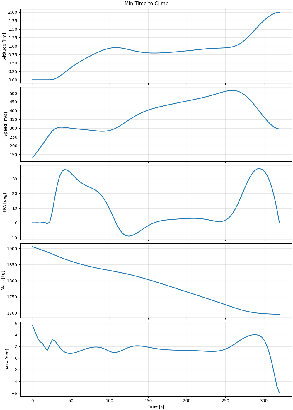
The optimized trajectory trades thrust, lift, drag, gravity, and fuel consumption to satisfy the terminal altitude and speed requirements in minimum time. From a modeling perspective, the key feature of this example is the direct use of interpolation-based atmosphere, propulsion, and aerodynamic data inside the dynamic equations.

---

[1]. GPOPS-II, "Minimum Time to Climb," https://www.gpops2.com/Examples/MinimumTimetoClimb.html.