Simulink Deployment
This section describes how to call the generated code in Simulink.
Here we use a Windows system as an example to demonstrate how to call the generated code in Simulink. The usage on other platforms is similar; you only need to set the correct compiler and link libraries in Simulink.
We use the Trajectory Tracking Control Problem as an example. The file structure of this example is as follows:
working_dir/
├── traj_tracking/
│   ├── traj_tracking_prob.c
│   ├── traj_tracking_prob.h
│   ├── traj_tracking_solver.h
│   ├── libtraj_tracking_solver_static.lib
├── traj_tracking.py
├── traj_tracking_sim.slx
.
Where:
traj_tracking.pyis the model file, which defines the trajectory tracking control problem model and code generation settings (withplatformset to'windows-x86_64-mingw'(Windows platform), andlib_typeset to'static'(static library))traj_tracking/is the code generation directorytraj_tracking_sim.slxis the Simulink model file
Prerequisites
Select the MinGW compiler in Matlab so that the generated code can run in Simulink:
>> mex -setup
MEX configured to use 'MinGW64 Compiler (C)' for C language compilation.
The compiler selected in Matlab must be compatible with the generated solver library; otherwise, compilation errors will occur.
For example, the solver library generated with 'windows-x86_64-mingw' requires selecting the MinGW compiler in Matlab;
the solver library generated with windows-x86_64-msvc requires selecting the MSVC compiler in Matlab.
Mismatched compilers will cause compilation errors.
Using S-Function to Call Generated Code
Here we use the S-Function Builder to call the generated code. The specific steps are as follows:
- Open Simulink and create a new model
- Add an S-Function Builder block in Simulink and double-click to open it
- Include the solver header files in the S-Function Builder Editor
#include "traj_tracking_prob.h"
#include "traj_tracking_solver.h" - Add the solver library files in the S-Function Builder Libraries
- Add
traj_tracking/to the include path - Add
libtraj_tracking_solver_static.libto libraries - Add
traj_tracking_prob.cto source files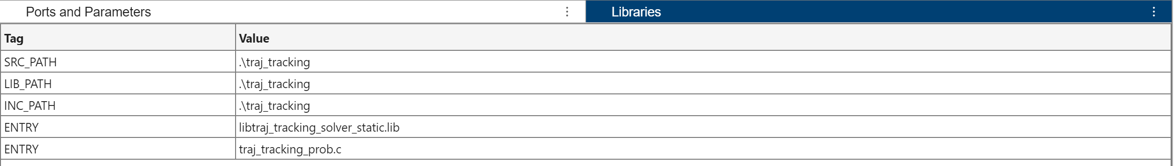
- Add
At this point, the inclusion of solver header files and library files in the S-Function Builder is complete. Below are the specific settings for the trajectory tracking control problem:
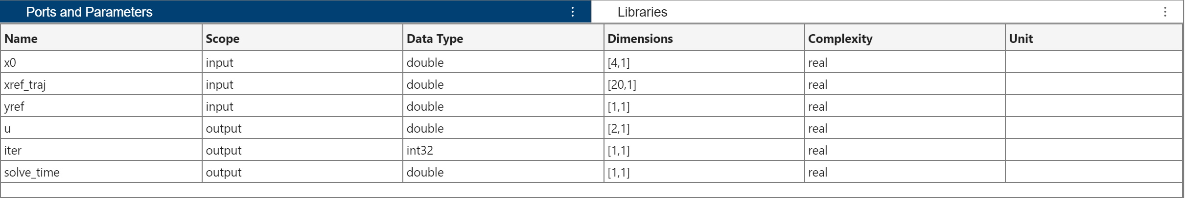
-
In the S-Function Builder's Ports and Parameters, define the input and output ports of the block. Here we define 3 input ports (x0, xref_traj, yref) and 3 output ports (u, iter, solve_time):
-
Implement the initialization, solving, and termination functions for the trajectory tracking controller in the S-Function Builder Editor
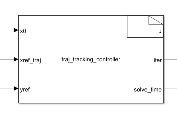
-
Click the Build button to generate the S-Function block:
Below is the complete code entered in the S-Function Builder Editor:
/* Includes_BEGIN */
#include "traj_tracking_prob.h"
#include "traj_tracking_solver.h"
#include <math.h>
/* Includes_END */

/* Externs_BEGIN */
static Traj_tracking_Problem prob;
static Traj_tracking_Option option;
static Traj_tracking_WorkSpace ws;
static Traj_tracking_Output output;
/* Externs_END */

void traj_tracking_controller_Start_wrapper(void)
{
/* Start_BEGIN */
    traj_tracking_init(&prob, &option, &ws);
    option.print_level = 0;
    option.try_warm_start_barrier = 1;
/* Start_END */
}

void traj_tracking_controller_Outputs_wrapper(const real_T *x0,
                                              const real_T *xref_traj,
                                              const real_T *yref,
                                              real_T *u,
                                              int32_T *iter,
                                              real_T *solve_time)
{
/* Output_BEGIN */
    const double vref = 1.0;
    const double ts_discretization = 0.2;
    /* params */
    prob.param[TRAJ_TRACKING_PARAM_XWEIGHT] = 1.0;
    prob.param[TRAJ_TRACKING_PARAM_YWEIGHT] = 1.0;
    prob.param[TRAJ_TRACKING_PARAM_VWEIGHT] = 1.0;

    // initial state
    prob.param[TRAJ_TRACKING_PARAM_X0] = x0[0];
    prob.param[TRAJ_TRACKING_PARAM_Y0] = x0[1];
    prob.param[TRAJ_TRACKING_PARAM_PHI0] = x0[2];
    prob.param[TRAJ_TRACKING_PARAM_V0] = x0[3];

    // reference trajectory
    prob.param[TRAJ_TRACKING_PARAM_VREF] = vref;
    for (size_t i = 0; i < TRAJ_TRACKING_DIM_N; i++) {
        prob.param_stage[i][TRAJ_TRACKING_PARAM_STAGE_XREF] = xref_traj[i];
    }
    prob.param[TRAJ_TRACKING_PARAM_YREF] = yref[0];

    // solve
    traj_tracking_solve(&prob, &option, &ws, &output);

    u[0] = output.primal.var[0][TRAJ_TRACKING_VAR_A];
    u[1] = output.primal.var[0][TRAJ_TRACKING_VAR_DELTA];

    iter[0] = output.iter;

    solve_time[0] = output.solve_time;
/* Output_END */
}

void traj_tracking_controller_Terminate_wrapper(void)
{
/* Terminate_BEGIN */

/* Terminate_END */
}
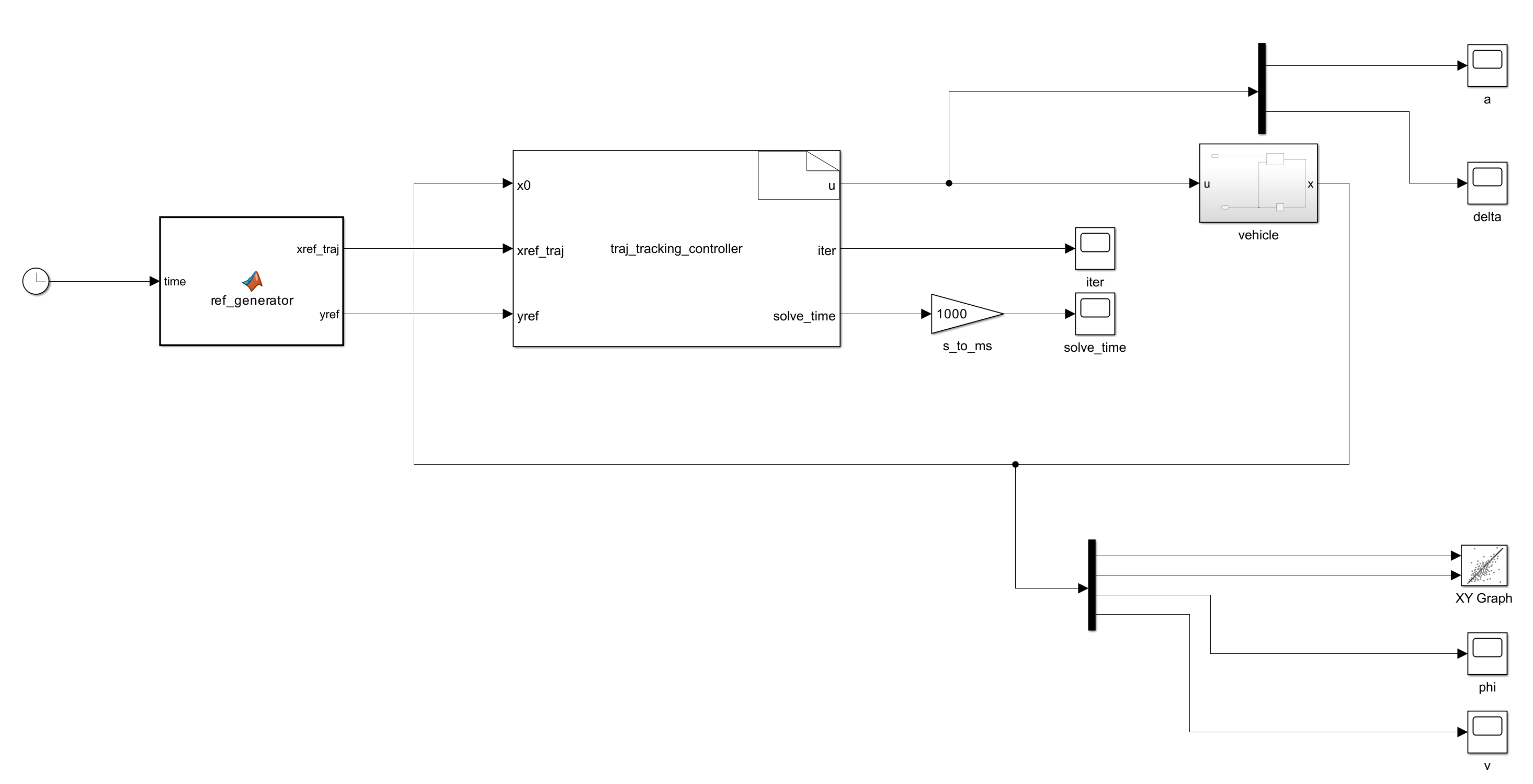
Running the Simulink Model
After completing the S-Function setup and building the closed-loop simulation for the trajectory tracking control problem, run the Simulink model.
The overall closed-loop simulation block diagram is shown below:
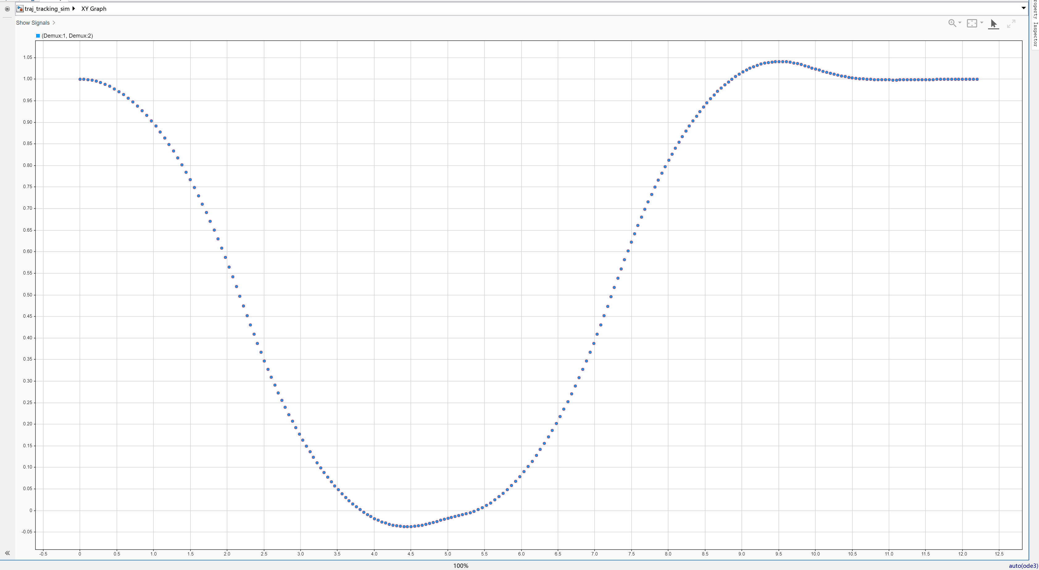
The closed-loop simulation trajectory is shown below:
Appendix
The following are the files used in this section:
You need to run traj_tracking.py to generate the code, then open the traj_tracking_sim_2017a.slx file in Simulink and run the simulation.